How to use XLOOKUP Formula in Excel?
XLOOKUP Formula in Excel is one of the Lookup & Reference Formula in Excel. The XLOOKUP Formula in Excel is used to search data in a table or range by row.
The article in this webpage describes how to use XLOOKUP formula in Excel with syntax, detailed explanation and examples.
What is XLOOKUP Formula in Excel?
The XLOOKUP Formula in Excel is one of the powerful formula which can search from right to left or left to right based on user defined criterias. The XLOOKUP Formula in Excel is the most flexible formula which can perform as a combination of multiple formulas and can replace them easily with better result.
The XLOOKUP Formula is not available in old Excel versions, so you must upgrade to the latest version of Excel to use it.
What is the Syntax of XLOOKUP Formula in Excel?
The Syntax of XLOOKUP Formula in Excel is:
=XLOOKUP(lookup_value, lookup_array, return_array, [if_not_found], [match_mode], [search_mode])
What are the Arguments of XLOOKUP Formula in Excel?
The Arguments of XLOOKUP Formula in Excel are explained below in detail and summary for your easy reference:
Lookup_Value (Required Argument)
This is the value you are searching. If it is omitted, then considered as blank cells.
Lookup_Array (Required Argument)
This is the array or range of the data to search.
Return_Array (Required Argument)
This is the array or range of the data to return.
[If_Not_Found] (Optional Argument)
This is the user defined value to return when a valid match is not found. If no value is defined then results as #N/A error.
[Match_Mode] (Optional Argument)
This is the match type which user can specify based on the below (if its omitted then considered as 0 by default for exact match):
- 0: Exact match (default)
- -1: Exact match or next smaller item
- 1: Exact match or next larger item
- 2: Wildcard character match
[Search_Mode] (Optional Argument)
This is the search type which user can specify based on the below:
- 1: Search first-to-last (default)
- -1: Search last-to-first
- 2: Binary search (sorting ascending order)
- -2: Binary search (sorting descending order)
Summary of Arguments:
- Lookup Value (Required) – value searching for.
- Lookup Array (Required) – range to search.
- Return Array (Required) – range to return.
- If Not Found (Optional) – if no match.
- Match Mode (Optional) – matching type of -1, 0, 1 and 2.
- Search Mode (Optional) – searching mode of 1, -1, 2 and -2.
What are the Advantages of XLOOKUP Formula in Excel?
The XLOOKUP Formula in Excel has many advantages over the other lookup formulas in Excel. Let’s find out in which ways XLOOKUP is better:
Search in Any Direction
In XLOOKUP formula, you can search the required result from left to right, right to left, ascending order or descending order.
User Defined Result if Error in Formula
The IFERROR formula in Excel is used along with other formula to replace the specified value if the formula returns an error. In XLOOKUP formula itself you can specift the value if the formula returns an error without using the IFERROR formula.
Multiple Results
By using the XLOOKUP formula’s return array argument, the user can get the entire row or column value easily instead of just one value. This is one of the unique advantage of using the XLOOKUP formula as compared to the old lookup formulas.
To understand the advantages of XLOOKUP formula in a better way, you must check below for VLOOKUP vs XLOOKUP formula in Excel.
What is the difference between VLOOKUP and XLOOKUP Formula in Excel? [VLOOKUP vs XLOOKUP]
The XLOOKUP Formula in Excel is new as compared to the old popular VLOOKUP Formula. The main differences between VLOOKUP and XLOOKUP Formula in Excel are:
Vertical or Horizontal Lookup
The VLOOKUP and HLOOKUP formulas in Excel are used for vertical and horizonal lookup respectively. But the XLOOKUP formula can also be used for vertical and horizonal lookup with better ways and returns the result easily.
Exact Match
For the match type in VLOOKUP formula there are two options (0/False for exact match and 1/True for approximate match). Whereas in XLOOKUP formula there are four options (0 for exact match, -1 for exact match or next smaller item, 1 for exact match or next larger item and 2 for wildcard match).
Search Right to Left
The VLOOKUP formula is used to search the data left to right and searching from right to left was a dream. The XLOOKUP formula solved this problem and can search the data in reverse order also i.e. from right to left or left to right.
First or Last Result
The VLOOKUP formula always gives the first search result from the array of information. Whereas in XLOOKUP formula the user can specify whether to get the first or last item.
Column Number
In VLOOKUP formula, the column number is one of the required argument and without this the user can not get the result. So, in VLOOKUP the user can either count the coulmn number manually or use the COLUMN formula to do the same. Whereas in XLOOKUP formula, the coulmn number is not required and the user can directly select the return array to get the result from that column.
Add or Delete Columns
If the user adds or deletes any column in the data after the VLLOKUP formula then the result will change and the user has to fix the coulmn number again. In XLOOKUP formula, this problem will not arise as its not dependent on the column number.
Speed
The VLOOKUP formula contains the entire table in the calculation from left to right, due to which it may slow down the Excel file. Whereas the XLOOKUP formula’s required arguments contain only lookup and return arrays instead of entire range.
Flixibility
The arguments of VLOOKUP formula are limited and defined to find things in a table by row. Whereas the XLOOKUP formula is more flexible to use with many arguments and the user can search with multiple conditions.
What is the difference between INDEX MATCH and XLOOKUP Formula in Excel? [INDEX MATCH vs XLOOKUP]
The INDEX MATCH is the combination for two formulas (INDEX and MATCH formula), which is commonly used after VLOOKUP formula and can solve difficult lookup problems.
After the XLOOKUP formula is introduced, its much better than INDEX MATCH formula and is more widely used due its advantages over the other lookup formulas. Let’s find out the difference between INDEX MATCH and XLOOKUP formula in Excel:
Complexity
The XLOOKUP formula is much easier to configure because you have to use one formula, whereas in INDEX MATCH you need to combine two formulas which makes it more complex.
Manage Error
The “if not found” argument in the XLOOKUP formula handles if there is an error in formula, whereas there is no such built in argument in INDEX MATCH formula.
Matching
The matching concept in XLOOKUP is much easy and simple as compared to INDEX MATCH formula.
Multiple Criterias
The XLOOKUP formula can handle multiple criterias and is much advanced as compared to the INDEX MATCH formula.
How to use XLOOKUP Formula in Excel with Examples?
Example 1 (Required Arguments)
In the below XLOOKUP example, the lookup_value is ST-04, lookup_array is ST. ID (B column) and return_array is Math (D column). The XLOOKUP formula in cell I5 returns 82, which is the mark for student ID ST-04.
=XLOOKUP(H5,B:B,D:D)
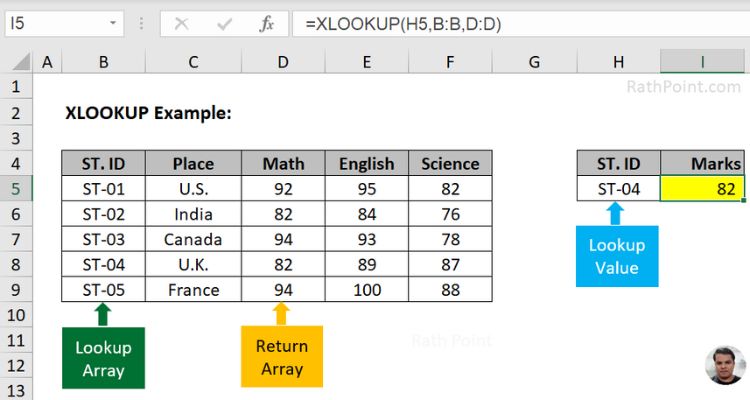
XLOOKUP Example 01 (Required Arguments)
Example 2 [if_not_found]
The [if_not_found] argument is optional and the user can define any value to return when a valid match is not found.
In the below XLOOKUP example, the Studend ID of ST-06 is not available in B column so the formula in cell I5 results as #N/A error.
=XLOOKUP(H5,B:B,D:D)
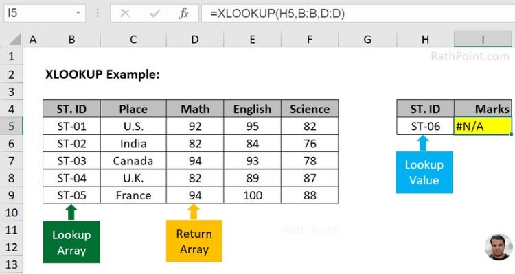
XLOOKUP Example 02 [if_not_found]
In the next XLOOKUP example, instead #N/A error let’s add the [if_not_found] argument with text as “No ST. ID” to return the same.
=XLOOKUP(H5,B:B,D:D,“No ST. ID”)

XLOOKUP Example 02 [if_not_found]
Example 3 [match_mode]
The [match_mode] argument is optional and the user can define 0, -1, 1 or 2. Let’s use all these match modes in the XLOOKUP formula and find out the results.
-1: Exact match or next smaller item
In this XLOOKUP example, the -1 for [match_mode] argumnet considered the next smaller item i.e. Studend ID 05 (ST-05) since the Studend ID 06 (ST-06) is not available.
=XLOOKUP(H5,B:B,D:D,”No ST. ID”,-1)
![XLOOKUP Formula in Excel - XLOOKUP Example 03 - [match_mode] -1 XLOOKUP Formula in Excel - XLOOKUP Example 03 - [match_mode] -1](https://rathpoint.com/wp-content/uploads/2023/11/XLOOKUP-Formula-in-Excel-XLOOKUP-Example-03-match_mode-1.jpg)
XLOOKUP Example 03 [match_mode] “-1“
1: Exact match or next larger item
In this XLOOKUP example, the 1 for [match_mode] argumnet considered the next larger item i.e. Studend ID 01 since the exact match (Studend ID 00) is not available.
=XLOOKUP(H5,B:B,D:D,”No ST. ID”,1)
![XLOOKUP Formula in Excel - XLOOKUP Example 03 - [match_mode] 1 XLOOKUP Formula in Excel - XLOOKUP Example 03 - [match_mode] 1](https://rathpoint.com/wp-content/uploads/2023/11/XLOOKUP-Formula-in-Excel-XLOOKUP-Example-03-match_mode-1-1.jpg)
XLOOKUP Example 03 [match_mode] “1“
2: Wildcard character match
In this XLOOKUP example, the 2 for [match_mode] argumnet considered wildcard feature with star (*5 in cell H5) and provides the results for Studend ID 05.
=XLOOKUP(H5,B:B,D:D,”No ST. ID”,2)
![XLOOKUP Formula in Excel - XLOOKUP Example 03 - [match_mode] 2 XLOOKUP Formula in Excel - XLOOKUP Example 03 - [match_mode] 2](https://rathpoint.com/wp-content/uploads/2023/11/XLOOKUP-Formula-in-Excel-XLOOKUP-Example-03-match_mode-2.jpg)
XLOOKUP Example 03 [match_mode] “2“ (wildcard)
0: Exact match (default)
In this XLOOKUP example, the 0 for [match_mode] argumnet considered the exact match and its the deafult even if ignored.
=XLOOKUP(H5,B:B,D:D,”No ST. ID”,0)
![XLOOKUP Formula in Excel - XLOOKUP Example 03 - [match_mode] 0 XLOOKUP Formula in Excel - XLOOKUP Example 03 - [match_mode] 0](https://rathpoint.com/wp-content/uploads/2023/11/XLOOKUP-Formula-in-Excel-XLOOKUP-Example-03-match_mode-0.jpg)
XLOOKUP Example 03 [match_mode] “0“
Example 4 [search_mode]
The [search_mode] argument is optional and the user can define 1, -1, 2 or -2. Let’s use few of these search modes in the XLOOKUP formula and find out the results.
-1: Search last-to-first
In this XLOOKUP example, both row 6 and 8 contains data for Student ID 04 (ST-04). The -1 for [search_mode] argumnet searched from last to first and provides the result found in row 8 (86 marks in Math).
=XLOOKUP(H5,B:B,D:D,”No ST. ID”,0,-1)
![XLOOKUP Formula in Excel - XLOOKUP Example 04 - [search_mode] -1 XLOOKUP Formula in Excel - XLOOKUP Example 04 - [search_mode] -1](https://rathpoint.com/wp-content/uploads/2023/11/XLOOKUP-Formula-in-Excel-XLOOKUP-Example-04-search_mode-1.jpg)
XLOOKUP Example 04 [search_mode] “-1“
1: Search first-to-last (default)
In this XLOOKUP example, the 1 for [search_mode] argumnet searched from first to last and provides the result found in row 6 (90 marks in Math).
=XLOOKUP(H5,B:B,D:D,”No ST. ID”,0,1)
![XLOOKUP Formula in Excel - XLOOKUP Example 04 - [search_mode] 1 XLOOKUP Formula in Excel - XLOOKUP Example 04 - [search_mode] 1](https://rathpoint.com/wp-content/uploads/2023/11/XLOOKUP-Formula-in-Excel-XLOOKUP-Example-04-search_mode-1-1.jpg)
XLOOKUP Example 04 [search_mode] “1“
Example 5 (Multiple Results)
The XLOOKUP formula in Excel can return an array with multiple items. In the below XLOOKUP example, the [return_array] is column D to E and returns the Math and English marks for Studend ID 04. The XLOOKUP formula in cell H5 is:
=XLOOKUP(G5,B:B,D:E)
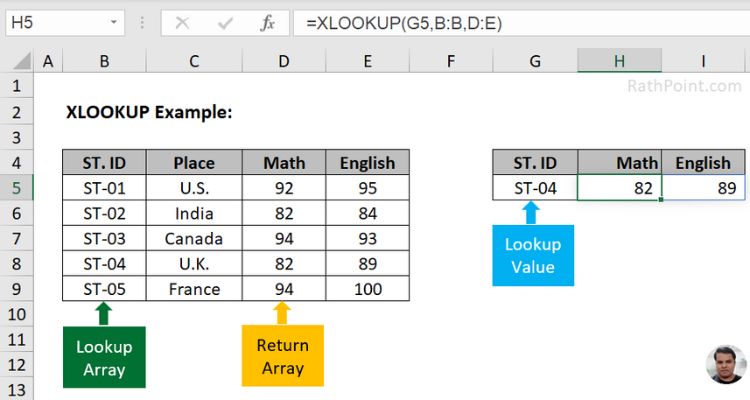
XLOOKUP Example 05 (multiple results)
Example 6 (replace HLOOKUP)
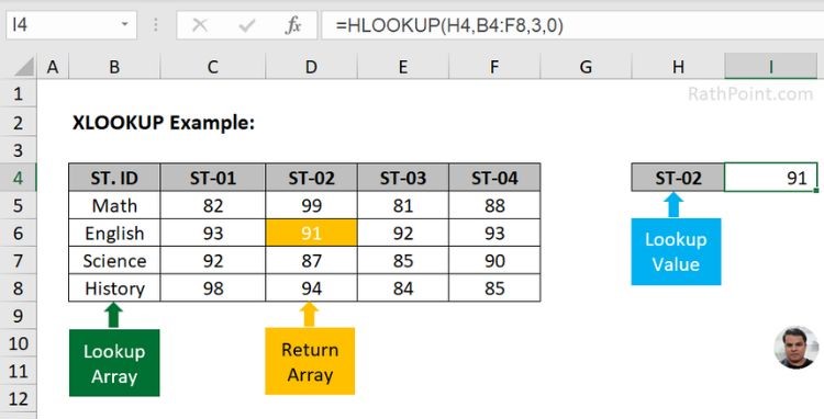
The XLOOKUP formula in Excel can easily replace the HLOOKUP formula also for horizontal lookup. Let’s learn HLOOKUP vs XLOOKUP formula with examples. The XLOOKUP formula in cell I4 to find the English mark for Studend ID 02 is:
=XLOOKUP(H4,B4:F4,B6:F6)
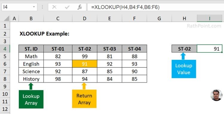
XLOOKUP Example 06 (replace HLOOKUP)
The above XLOOKUP formula is easy, whereas the HLOOKUP formula is complex and needs more information to fulfil the same need. To get the above result, the HLOOKUP formula in cell I5 is:
=HLOOKUP(H4,B4:F8,3,0)
XLOOKUP Example 06 (replace HLOOKUP)
Example 7 (Nested XLOOKUP)
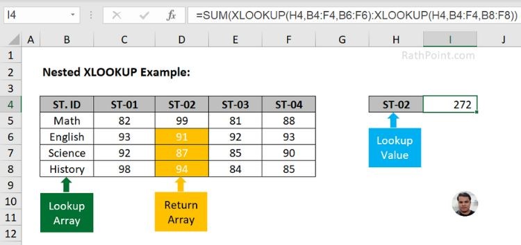
Multiple nested XLOOKUP formulas can be used as a range for sum or any other calculation. The XLOOKUP formula in cell I4 to sum the marks from English to History for Studend ID 02 is:
=SUM(XLOOKUP(H4,B4:F4,B6:F6):XLOOKUP(H4,B4:F4,B8:F8))
XLOOKUP Example 07 (nested XLOOKUP)
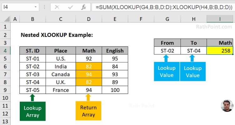
Let’s take another example for multiple nested XLOOKUP formulas to understand in a better way. The XLOOKUP formula in cell I4 to sum the marks of Math from Student ID 02 to 04 (ST-02 to ST-04) is:
=SUM(XLOOKUP(G4,B:B,D:D):XLOOKUP(H4,B:B,D:D))
XLOOKUP Example 07 (nested XLOOKUP)
What are the Key Points for XLOOKUP Formula in Excel?
You must remember the below key points while using the XLOOKUP formula in Excel:
- Ommit Lookup Value: If lookup_value is omitted, then the XLOOKUP formula returns the value of blank cells.
- #NAME Error: The XLOOKUP formula does not support in old Excel versions and you will get #NAME error.
- #VALUE Error: The user can define different ranges for the [return_array], but it must be within the same range limit else returns as #VALUE error in XLOOKUP formula.
- #NA Error: The #N/A error occurs in the Excel XLOOKUP Formula if the arguments are not defined properly and some of the additional causes are:
- Match not found and nothing is defined in [if_not_found].
- Exact match not found in [match_mode].

How to use XLOOKUP Formula in Excel?
» Excel Home
» Excel Formulas
» Financial Formulas
» Logical Formulas
» Text Formulas
» Date & Time Formulas
» Lookup & Ref Formulas
» Math & Trig Formulas
» Statistical Formulas
» Engineering Formulas
» Cube Formulas
» Information Formulas
» Compatibility Formulas
» Web Formulas
