How to use Conditional Formatting in Excel
Conditional Formatting in Excel is a powerful feature enabling users to dynamically adjust cell formats based on predefined criteria or rules. Whether aiming to emphasize crucial data points, detect trends, or conduct visual analyses of spreadsheets, the conditional formatting in Microsoft Excel significantly enhances efficiency by automatically implementing formatting styles. By defining conditions and rules, users can effortlessly tailor the presentation of their data, enhancing its clarity and visual impact. In this guide, we’ll show you how to use conditional formatting in Excel step by step.
What is Conditional Formatting in Excel?
The conditional formatting in Excel is like giving your spreadsheet special instructions to automatically format the cells based on rules you set. You can tell Excel, “If this happens, then do that.” For example, if a number is greater than 10, make the cell color as red.
Let’s understand the three fundamental elements constituting each conditional formatting rule in Excel:
- Cell Range: The cell range or array can be from a single cell to multiple cells across rows and columns.
- Condition: When you use the “if” part, you’re basically choosing from various options like “greater than,” “less than,” “between,” and more to define the conditions under which something should happen.
- Formatting: Its the formatting part, which will happen based on the condition(s) specified in the rule. The formatting includes changing color, font, border etc.
How to apply Conditional Formatting in Excel?
Follow the below steps to apply conditional formatting in Excel:
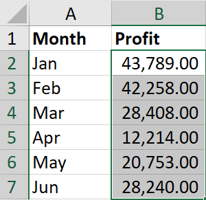
- Select Cells: Select the cell or range of cells where you want to apply conditional formatting. In this example, let’s select the cell range from B2 to B7.

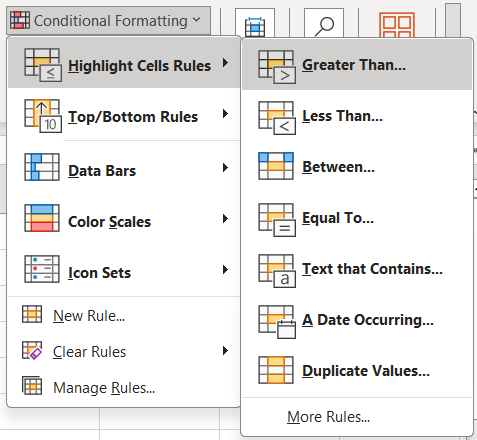
- Navigate to Conditional Formatting Icon: Go to the “Home” tab on the Excel ribbon, click on the “Conditional Formatting” icon in the “Style” group.
- Select Conditional Formatting Type: You can select the predefined conditional formatting options or create new rule. To understand, let’s click on “Highlight Cell Rules” ⇒ “Greater Than”.

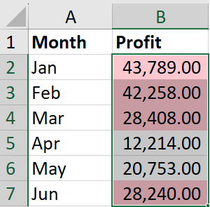
- Define Condition and Formatting: You can format the cells that are greater than the specified amount with specified formats. First define the amount based on which the greater than will be calculated (for example, 15,000). Next, either select the predified formats or click on custom format to apply based on your requirement (for example, Light Red Fill).

- Apply Conditional Formatting: Once you have defined the condition and format, click “OK” to apply it to the selected cells. In this example, based on the specified condition (greater than 15,000), the conditional formatting (Light Red Fill) applied.

How to apply Conditional Formatting in Excel using Shortcuts?
Below are the keyboard shortcut keys to apply conditional formatting in Excel:
Conclusion
Using conditional formatting in Microsoft Excel is like adding magic to your spreadsheets. It’s a powerful tool that helps you make your data look better and work smarter. With conditional formatting, you can easily highlight important numbers, spot trends, and make critical information stand out. You can do things like coloring, adding progress bars, or even creating your own rules based on your data.
So, take some time to explore Excel’s conditional formatting features and see how they can help you turn boring data into valuable insights.
Learn More
» How to Add Borders in Excel?
» How to Format Numbers in Excel?
» How to Format Font in Excel?
» How to Format Alignment in Excel?

Excel Tutorial Part 1 (Basic)
» Excel Home
» Excel Basics
» Excel Workbook
» Excel Template
» Excel Cell
» Excel Password
Excel Tutorial Part 2 (Format)
» Excel Clipboard
» Excel Format Font
» Excel Format Alignment
» Excel Format Number
» Excel Border
» Excel Conditional Formatting
Excel Tutorial Part 3 (Data)
» Excel Sort Data
» Excel Filter Data
» Excel Text to Columns
» Excel Data Validation
» Excel Flash Fill
» Excel Remove Duplicates
» Excel Relationships
» Excel Consolidate
» Excel What-If Analysis
» Excel Group
» Excel Charts
» Excel Table
» Excel PivotTable
Excel Tutorial Part 4 (Find)
» Excel Find and Replace
» Excel Go To
» Excel Select Objects
» Excel Selection Pane
Excel Tutorial Part 5 (Review)
» Excel Spell Check
» Excel Smart Lookup
» Excel Translate
» Excel Comments & Notes
» Excel Protect
» Excel Hide Ink
Excel Tutorial Part 6 (View)
» Excel Workbook Views
» Excel Formula Bar
» Excel Zoom
» Excel Window
» Excel Macros
Excel Tutorial Part 7 (Fx)
» Excel Formulas (Category)
» Excel Formulas (Alphabetical)
» Excel Errors
» Excel Name Manager
» Excel Formula Auditing
» Excel Watch Window
» Excel Calculation Options
Excel Tutorial Part 8 (Other)
» Excel Add-ins
» Excel Shortcuts

0 Comments