How to Create a Pivot Table in Excel

This guide will show you how to create a Pivot Table in Excel. The Pivot Table in Excel lets you quickly summarize and analyze large sets of data. It allows you to easily rearrange and view your data in different ways, helping you spot trends and patterns. With the help of a Pivot Table, you can turn your data into useful insights with just a few clicks, without changing the original data.

Why to Create a Pivot Table in Excel?

Before knowing how to create a Pivot Table in Excel, its importnt to learn why to create a Pivot Table in Excel. Below are some of the main reasons for creating the Pivot Table, which makes it one of the key fatures of the Microsoft Excel application, used to extract valuable insights and inform decision-making processes.

1. Summarized Data

The Pivot Table in Excel enables rapid summarization of large datasets. By simply dragging and dropping the headers to the fields, you can summarize the data in various ways without using complex formulas.

2. Simplified Data Organization

The Excel Pivot Table helps to organize and categorize data efficiently. Group data by various criteria like dates, categories, or other fields, making it easier to identify trends and patterns.

3. Versatile Data Analysis

The Pivot Table in Excel is extremely flexible. You can easily pivot (rearrange) the table to view data from different perspectives, such as switching rows and columns or filtering data to focus on specific segments.

4. Enhanced Reporting Capabilities

The Pivot Tables is a powerful tool for creating detailed and insightful reports. Features like conditional formatting and calculated fields allow you to highlight important data points and perform complex calculations on the fly.

5. Time Efficiency

The Pivot Table automates data analysis processes, reducing tasks that could take hours to mere minutes. This efficiency allows you to concentrate on interpreting data rather than processing it.

6. Interactive Data Exploration

You can create interactive reports and dashboards using the Pivot Table in Excel. Incorporate slicers and timelines to enable users to filter and drill down into the data dynamically, enhancing their data exploration capabilities.

7. Error Minimization

Manual data analysis can be prone to errors, especially with large datasets. The Pivot table can reduce the risk of errors by relying on consistent and structured data aggregation methods.

8. Data Integration

The Pivot Table can be used to handle data from various sources. You can easily consolidate the data from different sheets, workbooks, or even external databases, simplifying the analysis of combined datasets.

9. Data Visualization

You can link the Pivot Tables with pivot charts to provide a visual representation of the data. This aids in better understanding trends, outliers, and overall data distribution.

10. User Friendly Interface

Despite the powerful capabilities, the Pivot Tables are user-friendly. The Microsoft Excel provides a straightforward interface for creating and customizing the Pivot Tables, making them accessible even to users with limited technical expertise.

Steps: How to Create a Pivot Table in Excel?

Let’s understand how to create a Pivot Table in Excel in step by step.

Step 1: Select Data

• Select the entire data or click a cell within your data.
• Make sure your data is in a table with clear column names.
• Don’t leave any blank rows or columns in your data.
• Also, ensure your data in Excel is accurate and complete. Fix any mistakes or discrepancies in your data.
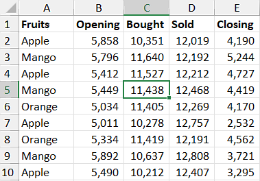
• In the below example, you can select the entire data range from A1 to E10 or just click a cell within it (C5).

Step 2: Access PivotTable Button

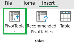
• Go to Insert tab in the ribbon and click on “PivotTable” button under Tables section.

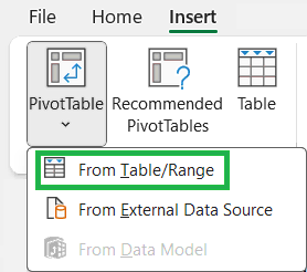
• Or, click the drop down arrow button under “PivotTable” and select “From Table/Range” option. If you want to create a Pivot Table in Excel from external data source or data model then you can select the required option.

Step 3: Create PivotTable from Table or Range

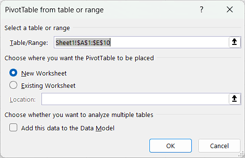
• Select the table o range from which you want to create a PivotTable in Excel.
• You have option to choose where you want the PivotTable to be placed, either in a new worksheet or in an existing worksheet.
• By default the new worksheet option will be selected. If you want in the existing worksheet then tick this option and select the cell where you want the PivotTable.
• Thenk click OK to create a Pivot Table in Excel.

Step 4: Choose PivotTable Fields

• You have to choose filelds to add to report and create PivotTable.

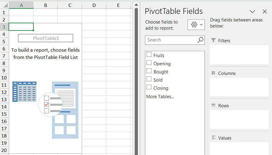
• To build a report, choose fields from the PivotTable Field List and drag fields between areas.
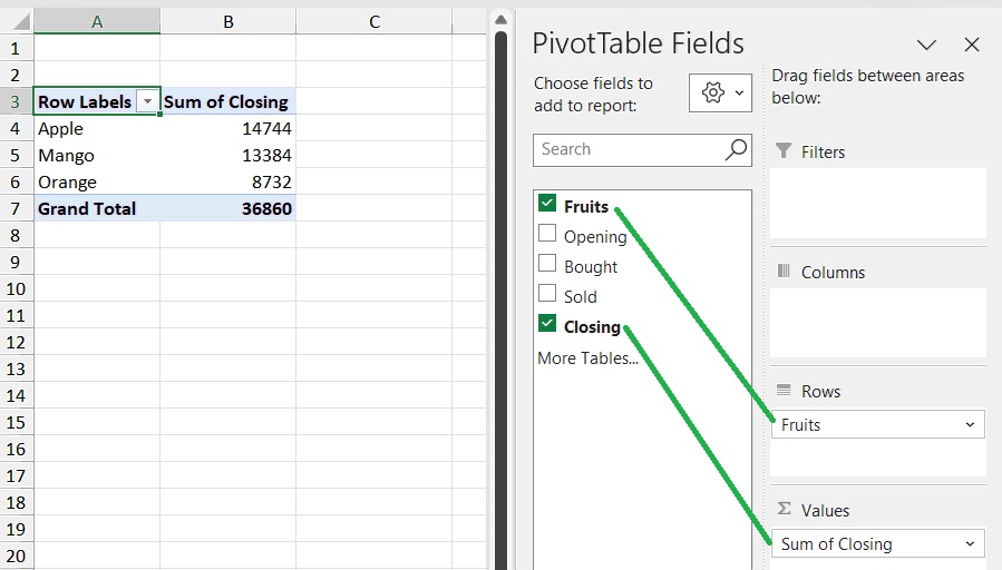
• For example, drag “Fruits” under rows and “Closing” under values section. Then the Pivot Table will be created in cell A3 to summarize the closing values of fruits from the data.
• To remove any field from any area, either remove the tick from the list or drag the field outside of the area. You can also move any field by dragging from one area to another.
• The data of the Pivot Table will change based on the fields you have selected and placed on the areas.

How to Create a PivotTable in Excel using Shortcuts?

Below is the keyboard shortcut key to create a Pivot Table in Excel:

Conclusion

In Excel, creating a Pivot Table is easy and helps you quickly summarize and analyze data. Just select your data range, go to the Insert tab, and choose PivotTable. You can place the Pivot Table in a new or existing worksheet. Then, drag fields into Rows, Columns, Values, and Filters to customize the table. This process turns raw data into clear insights, making it simpler to understand and present your results.

Learn More