How to use AMORLINC Formula in Excel?

AMORLINC formula in Excel is used to return the depreciation of an asset for each accounting period. The AMORLINC formula in Excel is a part of financial formulas.

The article in this webpage describes how to use AMORLINC formula in Microsoft Excel with syntax, detailed explanation and examples.

Subscribe Rath Point's official YouTube channel to know the latest updates, tips, and tricks.

What is AMORLINC Formula in Excel?

The AMORLINC formula in Excel calculates the depreciation of an asset for each accounting period on a prorated basis. The AMORLINC formula is provided for the French accounting system. In AMORLINC formula, the depreciation is prorated if the asset is purchased in the middle of the accounting period.

What is the Syntax of AMORLINC Formula in Excel?

The Syntax of Excel AMORLINC formula is:

=AMORLINC(cost, date_purchased, first_period, salvage, period, rate, [basis])

What are the Arguments of AMORLINC Formula in Excel?

The Arguments of AMORLINC formula in Microsoft Excel are explained below in detail and summary for your easy reference:

Cost (Required Argument)

This is the cost of an asset.

Date Purchased (Required Argument)

This is the asset’s date of purchase.

First Period (Required Argument)

This is the date of the end of the first period.

Salvage (Required Argument)

This is the asset’s salvage value at the end of the period.

Period (Required Argument)

This is the period for which the depreciation is calculated.

Rate (Required Argument)

This is the asset’s rate of depreciation.

Basis (Optional Argument)

This is the type of year basis to use for calculating depreciation. If you will omit the basis, then it will use zero (0) by default. You can use any one of the below basis:

• 0: US (NASAD) 30/360
• 1: Actual/actual
• 2: Actual/360
• 3: Actual/365
• 4: European 30/360

Summary of AMORLINC Arguments:

• Cost (Required) – cost of an asset.
• Date Purchased (Required) – date of purchase.
• First Period (Required) – end of first period.
• Salvage (Required) – salvage value.
• Period (Required) – period.
• Rate (Required) – depreciation rate.
• Basis (Optional) – year basis.

How to use AMORLINC Formula in Excel with Examples?

Example 1 (required arguments)

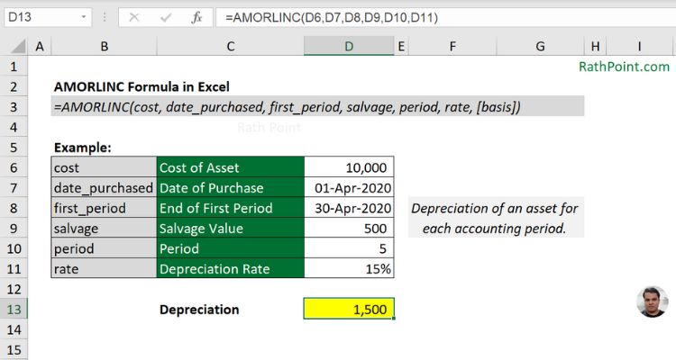
In the below example of AMORLINC formula in Excel, the depreciation for the asset is calculated as $1,500 by considering cost ($10,000), date of purchase (01-Apr-2020), first period (30-Apr-2020), salvage value (500), period (5 years) and depreciation rate (15%). The Excel AMORLINC formula in cell D13 is:

=AMORLINC(D6,D7,D8,D9,D10,D11)

Example 2 [basis]

The [basis] argument is optional in Excel AMORLINC formula and if you will ignore then it will consider as zero (0) by default and will use US (NASD) 30/360 for the same.

In the below AMORLINC formula example, the depreciation for the security is calculated as $1,200 by considering the [basis] argument as 1 (actual/actual) and keeping all other arguments same as shown in the previous AMORLINC formula example. The Excel AMORLINC formula in cell D14 is:

=AMORLINC(D6,D7,D8,D9,D10,D11,D12)

Example 3 (Dates)

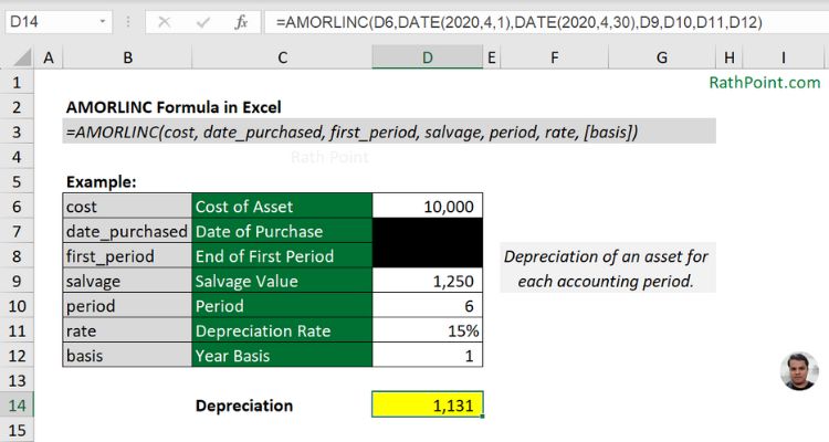
In AMORLINC formula, the dates should be entered in correct format and you can use the DATE formula also to avoid errors. The AMORLINC formula in cell D14 is:

=AMORLINC(D6,DATE(2020,4,1),DATE(2020,4,30),D9,D10,D11,D12)

What are the Key Points for AMORLINC Formula in Excel?

You must remeber the below key points while using the AMORLINC formula in Microsoft Excel:

• #NUM Error in the Excel AMORLINC formula, if:
  • rate <=0
  • salvage >= cost
  • basis <0 or >4
• Dates and basis are truncated to integers.