Excel TEXTSPLIT Function

The Excel TEXTSPLIT function splits text strings by using column and row delimiters. The Excel TEXTSPLIT function is a part of text formulas.

The TEXTSPLIT function is a dynamic and powerful tool for handling text data, introduced in Excel 365 and Excel 2019 as part of Excel’s dynamic array functions. The TEXTSPLIT function in Excel allows you to split text strings into multiple cells by defining specific delimiters, making it easy to manage and organize data without the complex formulas.

How to use the Excel TEXTSPLIT Function

The article in this webpage describes how to use the Excel TEXTSPLIT function with syntax, arguments, detailed explanation, and examples step by step.

TEXTSPLIT Syntax

=TEXTSPLIT(text, col_delimiter, [row_delimiter], [ignore_empty], [match_mode], [pad_with])

The arguments of TEXTSPLIT formula are:

• text (required) – Text you want to split.
• col_delimiter (required) – Specific character(s) used to split the text across columns.
• row_delimiter (optional) – Specific character(s) used to split the text across rows.
• ignore_empty (optional) – By default, FALSE or 0 (Zero) to create an empty cell. TRUE or 1 to ignore consecutive delimiters.
• match_mode (optional) – By default, 0 for case-sensitive match. Enter 1 for case-insensitive match.
• pad_with (optional) – By default, #N/A error for missing values. You can specify any value (like an empty string “”) in the place of missing values.

TEXTSPLIT Examples

Let’s understand the TEXTSPLIT formula in Excel with examples.

1. Split Text Horizontally to Columns

In Excel, to split the text of a cell into multiple columns, you can use the TEXTSPLIT formula. First select the cell with text, and then set the delimiter (col_delimiter) as the character or symbol based on which the split should happen.

For example, to split the text in cell A2 horizontally by commas, use the following formula in Excel:

=TEXTSPLIT(A2 , “,”)

The col_delimiter should be within the doubble quote. In this example the comma is the column delimiter, based on which the text is splitted (“,”).

The text in cell A2 is separated by a comma and the results are in cell C2 to E2.

You can use any other column delimiter based on which you want to split the text such as colon (“:”), semi-colon (“;”), hyphen (“-“), or empty space (” “).

2. Split Text Vertically to Rows

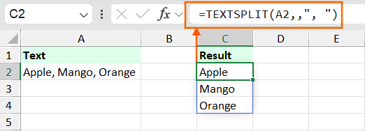
To separate the text of a cell into multiple rows, first select the cell with text, ignore the column delimiter (col_delimiter) by keeping comma (,), and then set the row_delimiter to split the text.

For example, to split the text in cell A2 vertically by comma and space, use the following formula in Excel:

=TEXTSPLIT(A2,,”, “)

In this example the comma and space (“, “) is the row delimiter, based on which the text in cell A2 is splitted, and the results are in cell C2 to C4.

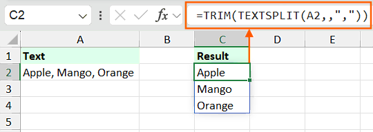
You can use the TRIM formula, instead of adding the space along with the delimiter. For example, to split the text in cell A2 vertically by comma and space, use the following alternative formula in Excel:

=TRIM(TEXTSPLIT(A2,,”,”))

In this example the comma (“,”) is the row delimiter, based on which the text in cell A2 is splitted, then the TRIM function removes the extra spaces, and the results are in cell C2 to C4.

3. Split Text to Columns and Rows

To split the text into columns and rows at the same time, specify both the col_delimiter and row_delimiter in the TEXTSPLIT function.

For example, to split the text in cell A2 across columns and rows, use the following formula in Excel:

=TEXTSPLIT(A2,”-“,”, “)

In this example the hyphen (“-“) is the col_delimiter, comma and space (“, “) is the row_delimiter, based on which the text in cell A2 is splitted, and the results are in cell C2 to D4.

4. Split Text by Multiple Delimiters

To split the text in a cell by multiple delimiters, use use an array constant like {“a”,”b”,”c”} for the column or row delimiter in the TEXSPLIT formula.

For example, to split the text in cell A2 across rows, use the following formula in Excel:

=TRIM(TEXTSPLIT(A2,,{“,”,”;”,”=”}))

In this example the row_delimiter contains comma (“,”), semi-colon (“;”) and equal sign (“=”), based on which the text in cell A2 is splitted, and the results are in cell C2 to C6.

Since, there is comma without space and with space, we have added the TRIM function to make it simple.

5. Split Text by Ignoring Empty Cells

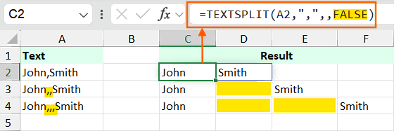
By default, the TEXTSPLIT function creates empty cells for consecutive delimiters. The ignore_empty argument is optional and if you ignore it, enter FALSE or 0 (zeor) then the results are same.

=TEXTSPLIT(A2,”,”)

Or

=TEXTSPLIT(A2,”,”,,FALSE)

In this example, we have used the col_delimiter as comma (“,”). But there are multiple commas in between the names in cell A3 and A4. Since we have entered FALSE in the ignore_empty argument, it splits the text based on each comma and we have empty cells in D3, D4 and E4.

In the TEXSPLIT function, if we will enter TRUE or 1 in the ignore_empty argument, then it will ignore the consecutive delimiters.

=TEXTSPLIT(A2,”,”,,TRUE)

In this TEXTSPLIT function example, we have enered the ignore_empty argument as TRUE. So, it ignores the empty cells by avoiding the consucutives delimiters. And the results in cell C2 to D4 are different as compared to the previous example.

6. Split Text by Case-sensitive or Case-insensitive

By default, the match_mode argument is 0, which makes the delimiter case-sensivive.

=TRIM(TEXTSPLIT(A2,”x”,”,”,TRUE,0))

In this example the row_delimiter is small x (“x”) and the match_mode argument is 0 (case-sensivive), due to which the text is not splitted in cell C3 as it contains capital X and returns error in cell D3.

To make TEXTSPLIT case-insensitive, set the match_mode argument to 1. This tells the TEXTSPLIT function to ignore differences in letter case when splitting text.

=TRIM(TEXTSPLIT(A2,”x”,”,”,TRUE,1))

In this example of TEXTSPLIT formula the match_mode argument is 1 (case-insensitive), due to which the text is splitted by ignoring the upper or lowercase of the delimiter. The text in cell A2 is splitted by the row_delimiter as x or X  (“x”), the col_delimiter as comma (“,”), and the results are in cell C2 to D4.

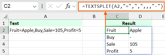
7. Split Text by Replacing Missing Values

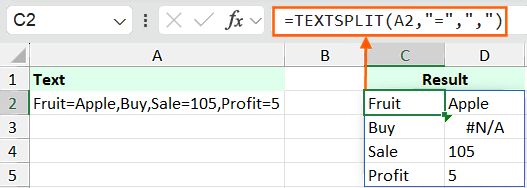
In TEXTSPLIT function, the pad_with is the last argument and is useful when some values are missing in the source text. When splitting a string into both rows and columns, if there are gaps in the data, the TEXTSPLIT function by default shows #N/A errors for those missing values.

=TEXTSPLIT(A2,”=”,”,”)

In this example the row_delimiter is small x (“x”) and the match_mode argument is 0 (case-sensivive), due to which the text is not splitted in cell C3 as it contains capital X and returns error in cell D3.

To make TEXTSPLIT case-insensitive, set the match_mode argument to 1. This tells the TEXTSPLIT function to ignore differences in letter case when splitting text.

=TEXTSPLIT(A2,”=”,”,”,,,”-“)

In this example of TEXTSPLIT formula the match_mode argument is 1 (case-insensitive), due to which the text is splitted by ignoring the upper or lowercase of the delimiter. The text in cell A2 is splitted by the row_delimiter as x or X  (“x”), the col_delimiter as comma (“,”), and the results are in cell C2 to D4.

Important Notes

• The TEXTSPLIT function is available in Microsoft Excel 365 (Office 365) and Excel for the Web.
• If you are using the old Excel version and the TEXTSPLIT function is not available, then use the Text to Columns feature to split the text.
• In reverse, to combine the text of multiple cells into a single cell with a specific delimiter, you can use the TEXTJOIN function in Excel.
• The TEXTSPLIT function in Excel can be used for various tasks, such as splitting names, dates, addresses, or any other data separated by delimiters into individual cells.

Learn More