How to use Advanced Filter in Excel
This guide will show you how to use advanced filter in Excel, so that you can manage and analyze data more effectively. In Excel, basic filters just help you filter, sort and show specific data. Advanced filters, on the other hand, let you use more complex criteria to find exactly what you want. They can also help you extract unique records and perform more detailed data tasks.
What is Advanced Filter in Excel?
The advanced filter in Excel is very helpful when working with large amounts of data, making it easy to find specific information. Whether you’re making reports, analyzing data in detail, or preparing data for other uses, learning to use advanced filter in Excel can make you more productive and improve your decision-making.
An advanced filter in Excel is a feature that gives you more options for filtering data. Unlike basic filter, which can only filter one condition per column, the advanced filter lets you use multiple criteria across different columns at the same time. This is useful for in-depth data analysis and creating detailed reports.
What are the Key Features of Advanced Filter in Excel?
- Multiple Criteria: You can set multiple rules for filtering your data. For example, filter rows where profits are more than $1000 and for April month.
- Complex Criteria: Use logical operators like AND and OR to combine rules. This allows more detailed filtering that basic filters can’t do.
- Copy to Another Location: The advanced filter lets you either filter the data in place or copy it to another location. This helps create custom reports without changing the original data.
- Unique Records Only: By using the advanced filter in Excel, you can show only unique entries from the filtered data and remove duplicate information.
How to use Advanced Filter in Excel with Multiple Criteria?
Follow the below steps to use advanced filter in Excel with multiple criteria:
- Select Data: Select the data in a cell range or table or click on any cell within the range of data where you want to apply the advanced filter. For example, from the below data either select the cell range A1 to D7 or click on any cell within this range.
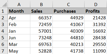
- Filter Icon: Go to the “Data” tab ⇒ “Sort & Filter” group and click on “Advanced” icon.
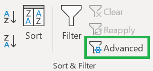
- Action and List Range: In advanced filter dialog box, by default the “Filter the list, in place” will be ticked under “Action’ section. The “List range” will automatically select the cell range if you have followed the first step, else you can click on the up arrow at the right hand side to select the range manually.
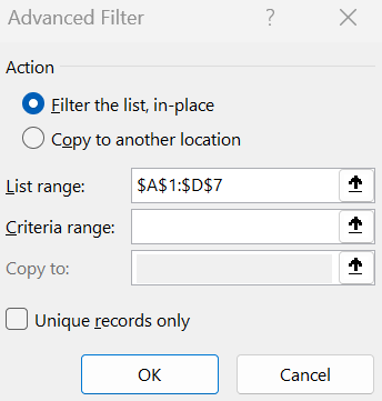
- Criteria Range: Select the criteria range based on which the advanced filter to be applied. Either you can type the criteria as show below or click on the arrow botton at the right side to select the criteria range.
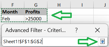
- Apply Advanced Filter: Once you have defined the action, range and criteria, click “OK” to apply the advanced filter to the selected cells. In this example, based on the list range ($A$1:$D$7) and criteria range (Sheet1!$F$1:$G$2), it will return the Feb month profits greater than $25,000.

How to use Advanced Filter in Excel with IF and OR criteria?
Let’s learn how to use the advanced filter with IF and OR criteria in Excel.
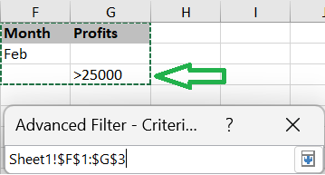
The OR criteria should be in the second line besides the first criteria. In the below example, the OR criteria is Profits greater than $25,000. You should select the criteria range from F1 to G3 to apply the OR criteria. If you will keep the second criteria (Profits greater than $25,000) in cell G2 then it will consider as AND criteria.
How to use Advanced Filter in Excel to Copy to Another Location?
Follow the below steps to copy advanced filtered data to anothere location or worksheet:
Step 1: First, go to the destination sheet and click on the cell where you want to copy the advanced filtered date. This step is important else you will get the error message.
Step 2: Go to the Data tab and click on Advanced icon under Sort & Filter group.
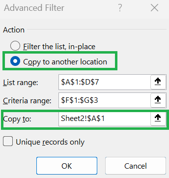
Step 3: In Advanced filter dialog box, select “copy to another location” under “Action” section.
Step 4: Select the entire table or date under “List range”. And select the conditions under the “Criteria range”.
Step 5: Select destination sheet’s cell under “Copy to” option and click “OK”.
How to fix Advanced Filter Errors in Excel?
There are multiple reasons for errors in advanced filter. In this guide we will explain the advanced filter errors and how to fix step by step.
The Extract Range has a Missing or Invalid Field Name
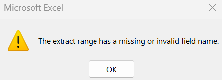
You will get error “The extract range has a missing or invalid field name” while using the advanced filter in Excel, if the “Copy to” cell reference is within the “List range”. So, change the “Copy to” path to an empty cell to get the issue fixed. Make sure you have enough empty cells where you want to copy the filtered data.
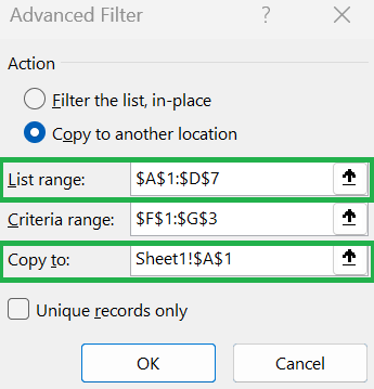
Also, make sure there are no merged cells and proper headers to work the advanced filter smoothly.
You Can Only Copy Filtered Data to the Active Sheet
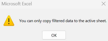
To avoid the error “You can only copy filtered data to the active sheet”, make sure first you go to the destination sheet’s cell and click on the cell where you want to copy the advanced filtered data. For example, if you want to copy advanced filtered data to Sheet 2 then first go to the Sheet 2 and click on cell A1.
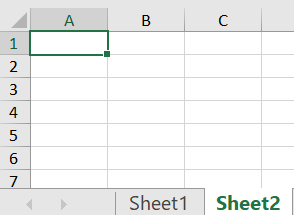
Then click on Advanced Filter icon and follow the below steps:
- Under action, click the “copy to another location”.
- Select the whole date under “List range” and conditions under the “Criteria range”.
- Select another sheet’s location or different cell of the same sheet under “Copy to” option.
- Click “OK” to apply the advanced filter.
How to use Advanced Filter in Excel by Shortcuts?
Below is the keyboard shortcut key to use advanced filter in Excel:
Conclusion
The Excel advanced filter lets you to quickly find specific information from large datasets using detailed criteria that regular filters can’t handle. With advanced filters, you can perform thorough searches, conduct in-depth analysis, and generate custom reports tailored to your needs. This saves time and improves the accuracy and usefulness of your data.
Learn More
» How to Filter Data in Excel?
» How to Sort Data in Excel?
» How to use Conditional Formatting in Excel?
» How to Add Borders in Excel?
» How to Format Numbers in Excel?
» How to Format Font in Excel?
» How to Format Alignment in Excel?

Excel Tutorial Part 1 (Basic)
» Excel Home
» Excel Basics
» Excel Workbook
» Excel Template
» Excel Cell
» Excel Password
Excel Tutorial Part 2 (Format)
» Excel Clipboard
» Excel Format Font
» Excel Format Alignment
» Excel Format Number
» Excel Border
» Excel Conditional Formatting
Excel Tutorial Part 3 (Data)
» Excel Sort Data
» Excel Filter Data
» Excel Text to Columns
» Excel Data Validation
» Excel Flash Fill
» Excel Remove Duplicates
» Excel Relationships
» Excel Consolidate
» Excel What-If Analysis
» Excel Group
» Excel Charts
» Excel Table
» Excel PivotTable
Excel Tutorial Part 4 (Find)
» Excel Find and Replace
» Excel Go To
» Excel Select Objects
» Excel Selection Pane
Excel Tutorial Part 5 (Review)
» Excel Spell Check
» Excel Smart Lookup
» Excel Translate
» Excel Comments & Notes
» Excel Protect
» Excel Hide Ink
Excel Tutorial Part 6 (View)
» Excel Workbook Views
» Excel Formula Bar
» Excel Zoom
» Excel Window
» Excel Macros
Excel Tutorial Part 7 (Fx)
» Excel Formulas (Category)
» Excel Formulas (Alphabetical)
» Excel Errors
» Excel Name Manager
» Excel Formula Auditing
» Excel Watch Window
» Excel Calculation Options
Excel Tutorial Part 8 (Other)
» Excel Add-ins
» Excel Shortcuts

0 Comments