How to use Formula Auditing in Excel

In this article, you will learn how to use Formula Auditing in Excel step by step.

Table of Contents:

What is Formula Auditing in Excel?

The formula auditing in Excel is a set of tools that helps to check, understand, and fix formulas in a spreadsheet. It shows how formulas are connected, helps find mistakes, and ensures calculations are correct. This is especially helpful for big spreadsheets with many formulas.

What are the Formula Auditing Tools in Excel?

The Formula Auditing tools in Excel are found in the Formulas tab, which consists of:

• Trace Precedents,
• Trace Dependents,
• Remove Arrows,
• Show Formulas,
• Error Checking,
• Evaluate Formula, and
• Watch Window.

Let’s learn all the Formula Auditing tools in Excel one by one in detail.

Trace Precedents

The Trace Precedents in Excel helps to track which cells contribute to the value of a selected cell. It draws arrows from the source cells to the dependent cell, making it easier to understand how data flows within your spreadsheet.

How to use Trace Precedents in Excel?

• Select the cell that contains the formula you want to examine.

• Click on the Formulas tab in the Excel ribbon.

• In the Formula Auditing group, click Trace Precedents.

• The Excel will draw arrows pointing to the cells that directly contribute to the selected cell’s value.

Example

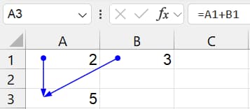
If a formula in A3 is =A1 + B1, clicking Trace Precedents on A3 will show arrows from A1 and B1.

What the Arrows Mean in Trace Precedents?

• The Blue arrows represent cells that provide input to the selected cell without errors.

• The Red arrows indicate an issue, such as an error in one of the precedent cells.

Trace Dependents

The Trace Dependents helps to see which other cells are affected by the value in a selected cell. It is useful when working with formulas because it shows how data flows through your spreadsheet.

How to use Trace Dependents in Excel?

• Click on the cell you want to check.

• Go to the Formulas tab at the top of Excel.

• Click on Trace Dependents in the Formula Auditing group.

• The arrows will appear, pointing to the cells that depend on the selected cell.

Example

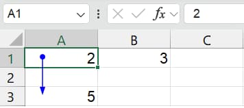
If a formula in A3 is =A1 + B2, clicking Trace Dependents on A1 will show an arrow to A3.

What the Arrows Mean in Trace Dependents?

• The Blue arrows show that the dependent cells are in the same worksheet.
• The Black dashed arrows indicate that the dependent cells are in another worksheet or a different file.
• If you see circular references, it means a formula is referring to itself, which can cause errors.

Remove Arrows

The Excel displays arrows when you use trace precedents or dependents tools in Formula Auditing. To remove the arrows in Excel:

• Go to the Formulas tab.

• Click Remove Arrows in the Formula Auditing group, 

Show Formulas

The Show Formulas in Excel allows to see the actual formulas inside the cells instead of their calculated results. This Formula Auditing tool in Excel helps to check and fix formulas in a spreadsheet.

How to Show Formulas in Excel?

• Click on the cell containing formula.

• Go to Formulas tab and look for the Formula Auditing section.

• Click on Show Formulas.

Excel Settings to Show Formulas Always in Windows OS

• Click on File in the top-left corner.
• Select Options from the menu.
• In the Excel Options window, click on Advanced from the left panel.
• Scroll down to the section called Display options for this worksheet.
• Check the box that says Show formulas in cells instead of their calculated results.
• Click OK.

Example

If a cell contains =2+3, Excel will show the result as 5. But if you turn on Show Formulas, you will see =2+3 in the cell instead of 5.

Error Checking

The Error Checking in Excel helps to systematically identify and resolve formula errors in a workbook. It acts like a spell checker for formulas, guiding users through each issue it detects, offering explanations, and in some cases, suggesting corrections.

How to use Error Checking in Excel?

• Go to the Formulas tab on the Excel Ribbon.
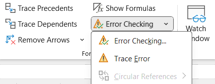
• Click on Error Checking in the Formula Auditing group.
• It scans the worksheet for any cells that contain formula errors and highlights them one at a time.

For each error found, the tool provides the following:

• Error Message: A brief description of the issue. For example:
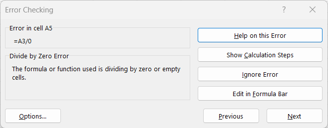
  • Error in cell A5: =A3/0.
  • Divided by Zero Error: The formula or function used is dividing by zero or empty cells.
• Help on this error: A link to detailed help documentation relevant to the specific error type.
• Show Calculation Steps: Opens the Evaluate Formula dialog box to walk through the formula’s logic.
• Ignore Error: Lets you dismiss the error if it’s expected or acceptable.
• Edit in Formula Bar: Takes you directly to the formula bar so you can correct the formula manually.
• Previous / Next: Navigate through multiple errors in your workbook.

Evaluate Formula

The Evaluate Formula in Excel lets you to check a formula step-by-step. It shows how Excel solves the formula, one part at a time. This is helpful when your formula has functions inside other functions, cell references, or if you’re not getting the result, you expected and want to find the mistake.

How to Evaluate Formula in Excel?

• Click on the cell that contains the formula you want to evaluate.
• Go to the Formulas tab on the ribbon.
• In the Formula Auditing group, click Evaluate Formula.
• The Evaluate Formula window will pop up showing your formula. You will find the first part of the formula is underlined — that’s what Excel will evaluate first.

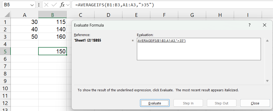
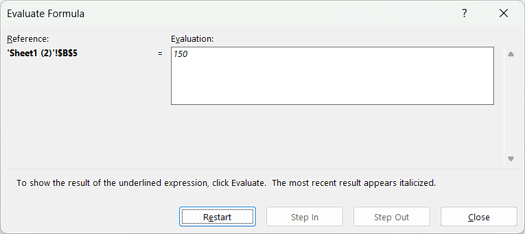
• Click Evaluate button to calculate the underlined part and it will replace with the result of that part.

• Each time you click on Evaluate button, it moves to the next part.

Watch Window

The Watch Window in Excel helps you to keep an eye on important cells, no matter where you are in your spreadsheet. If you are working on a big Excel file with lots of data in multiple sheets, it can be a pain to keep checking values such as formulas, links, totals etc., in the worksheets. You might have to scroll a lot or keep switching between sheets. That’s where the Watch Window becomes a handy tool to use.

How to use Watch Window in Excel?

• Go to the Formulas tab on the Ribbon.
• Click on Watch Window in the Formula Auditing group.

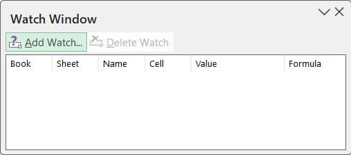
• In the Watch Window dialog box, click Add Watch.
• Select the cell or range of cells you want to monitor, then click Add.

• The selected cells will now be listed in the Watch Window, showing their current values and formulas.
• You can click the Close button when you do not need it anymore.

Why should you use Formula Auditing in Excel?

• Find mistakes: The formula auditing in Excel helps you to detect errors in formulas and correct them.
• See connections: The formula auditing tools in Excel shows which cells are used in a formula and which formulas depend on a specific cell.
• Check accuracy: You can easily verify that your calculations are correct in Microsoft Excel before using them for important decisions.
• Fix complex formulas: With the help of auditing tools in Excel, the long and difficult formulas can be broken down step by step to find and fix any issues.

Shortcut Keys

Below are the keyboard shortcut keys to use Formula Auditing tools in Excel:

Conclusion

The Formula auditing in Excel helps you check that your formulas are correct and working the way they should. It lets you see which cells are connected, find and fix errors, and understand how your calculations are done. The Excel Formula Auditing tools like Trace Precedents, Trace Dependents, Evaluate Formula, and Error Checking make it easier to find problems and fix them quickly. Using these tools saves time, helps avoid mistakes, and makes sure the Excel gives accurate results.

Learn More