GROUPBY Function in Excel

The GROUPBY function in Excel creates a summary of data via a formula. The GROUPBY function in Excel is a part of lookup and reference formulas.

The GROUPBY function organizes data by grouping rows based on given fields, applying aggregations (like SUM, AVERAGE, or COUNT), and sorting or filtering the results.

How to use GROUPBY Function in Excel

The article in this webpage describes how to use the GROUPBY function in Microsoft Excel with the syntax, arguments, detailed explanation, and examples step by step.

GROUPBY Syntax

=GROUPBY(row_fields, values, function, [field_headers], [total_depth], [sort_order], [filter_array], [field_relationship])

The arguments of GROUPBY function are:

• row_fields (required) – The range containing the values for grouping.
• values (required) – The range containing the values to aggregate.
• function (required) – The function used to do the aggregations.
• field_headers (optional) – A number between 0 and 3 that specifies whether the field data has headers and whether field headers should be returned in the results.
  • • Automatic (default): Excel to decide based on data.
    • 0: No headers.
    • 1: Yes – headers in data, but don’t show them.
    • 2: No headers in data, but Excel generates them.
    • 3: Yes – headers in data and show them.
• total_depth (optional) – to show the totals and subtotals at the bottom or top.
  • • 0: No Totals.
    • 1 (default): Grand Totals at the bottom.
    • 2: Grand and Subtotals at the bottom.
    • -1: Grand Totals at the top.
    • -1: Grand and Subtotals at the top.
• sort_order (optional) – A numeric value specifying the sort order for rows in Excel. Use positive numbers for ascending order sorting (default) and negative numbers for descending order sorting.
• filter_array (optional) – Logical expression to filter specific rows.
• field_relationship (optional) – Defines the relationship when multiple columns are in row_fields.
  • • 0: Hierarchy (default).
    • 1: Table.

GROUPBY Examples

Let’s understand the CODE function in Excel with examples.

1. Summary of Data

The GROUPBY function in Excel organizes rows in a specified array by grouping them based on the unique values and calculates a summary for each group.

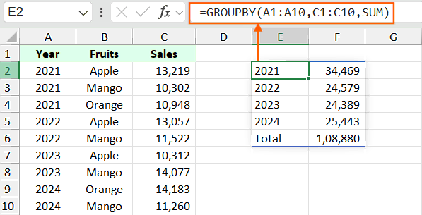
Let’s understand the Excel GROUPBY function with an example. Suppose you have a table of data as shown in the below image and you want the summary of sales based on the year, then the GROUPBY function in Excel will be:

=GROUPBY(A1:A10,C1:C10,SUM)

In this example, the row_fields is A1:A10 containing the years which you want to group, values in C1:C10 and the SUM function to total the values.

Apart from SUM, you can also use the other functions, such as PERCENTOF, AVERAGE, MEDIAN, COUNT, COUNTA, MAX, PRODUCT, ARRAYTOTEXT, CONCAT, STDEV.S, STDEV.P, VAR.S, VAR.P, MODE.SNGL, and LAMBDA.

2. Show Headers

By default, the GROUPBY function does not show the headers. To show the headers in the output, you need to use the argument field_headers in the GROUPBY function.

In the previous example the header was not visible. To show the header select the option 3 for the next argument fileld_headers and the GROUPBY formula will be:

=GROUPBY(A1:A10,C1:C10,SUM,3)

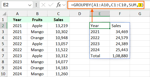
The above GROUPBY function will show headers only if your data contains the header.

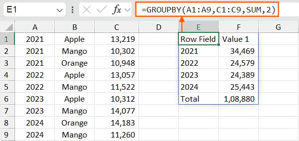
If the data is without headers then use the option 2, so that the Excel will auto generate the headers based on the data and the GROUPBY function will be:

=GROUPBY(A1:A9,C1:C9,SUM,2)

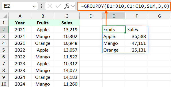
3. Show/Hide Totals

By default, the GROUPBY function shows the total at the bottom. The total_depth argument in GROUPBY function can be used to show or hide the totals and subtotals at the top or bottom.

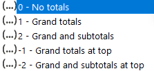
For example, you do not want to show the totals then the GROUPBY function will be:

=GROUPBY(B1:B10,C1:C10,SUM,3,0)

Important Notes

• The GROUPBY function, introduced in Excel 365 as part of dynamic array functions.
• The GROUPBY function is used to group data based on certain criteria and perform operations on the grouped data.
• The GROUPBY function returns #SPILL! error if any adjacent cells contain content, such as text, spaces, or hidden characters, as this prevents the formula from expanding its output into the blocked range.
• The GROUPBY function returns #VALUE! error if the ranges provided in between two arguments have mismatched.
• The GROUPBY function allows for aggregation and summarization of data in a more flexible and powerful way compared to the PivotTable.

Learn More