How to use IFERROR Formula in Excel?
The IFERROR formula in Excel returns user defined value if a formula error occurs. The IFERROR formula in Excel is a part of logical formulas.
The article in this webpage describes how to use IFERROR formula in Microsoft Excel with syntax, detailed explanation and examples.
Subscribe Rath Point's official YouTube channel to know the latest updates, tips, and tricks.
What is IFERROR Formula in Excel?
The IFERROR formula in Excel is used to trap and handle errors in a formula. The IFERROR formula returns the user specified value if a formula results to an error, otherwise returns the result of the formula. The IFERROR belongs to a group of error-checking formulas such as ISERR, ISERROR, IFNA and ISNA.
Sometimes you may get errors in formula due to multiple reasons. Instead of getting error message, you can define the specified result by using the IFERROR formula. The IFERROR formula can handle all types of errors in Excel due to formula such as “#N/A”, “#VALUE!”, “#REF!”, “#DIV/0!”, “#NUM!”, “#NAME?” and “#NULL!”. In this page, you will not find how to check errors in Excel, rather you will learn how to replace the formula errors with specified value to keep the data clean.
What is the Syntax of IFERROR Formula in Excel?
The syntax of IFERROR formula is as follows:
=IFERROR(value, value_if_error)
What are the Arguments of IFERROR Formula in Excel?
The arguments for IFERROR formula are explained below in detail and summary for your easy reference:
Value (Required Argument)
This is the formula or logical expression that needs to be checked for error.
Value if Error (Required Argument)
This is the user specified value to return if the formula error occurs.
IFERROR Arguments:
- Value (Required) – formula or expression.
- Value if Error (Required) – given value in case of error.
How to use Excel IFERROR Formula with Examples?
Example 1 (simple IFERROR formula)
In this simple division, there are errors in cell F7 and F8.
=C6/D6
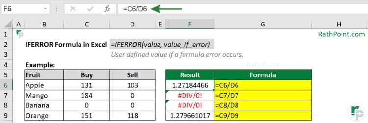
In the calculation, add the IFERROR formula and provide the specific value in case of error. In this IFERROR formula example, since we have defined as “0 buy/Sell” in case of error, we will get the same in case of “#DIV/0!” errors in cell F7 and F8.
=IFERROR(C6/D6,”0 Buy/Sell”)
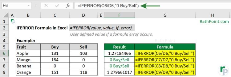
IFERROR formula Example (simple IFERROR formula)
Example 2 (#N/A Error)
The IFNA formula can handle only #N/A error, whereas the IFERROR formula can handle all types of errors such as #N/A, #VALUE!, #REF!, #DIV/0!, #NUM!, #NAME? and #NULL!.
Let’s understand with example, how the IFERROR formula can handle the #N/A error.
=VLOOKUP(“Cherry”,B5:D9,2,0)
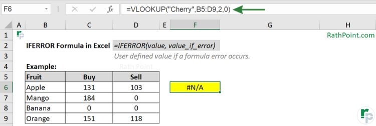
In the above VLOOKUP formula there is #N/A error which can be handled by the IFERROR formula. In the below IFERROR formula example, the text “Not Available” is specified in place of the #N/A error.
=IFERROR(VLOOKUP(“Cherry”,B5:D9,2,0),”Not Available”)

IFERROR formula Example (#N/A Error)
Example 3 (value)
In IFERROR formula, you can define the specified text, another formula or any value to handle all types of errors. In the below IFERROR example, the specified value is zero (0) which does not need any double quote.
=IFERROR(VLOOKUP(“Cherry”,B5:D9,2,0),0)
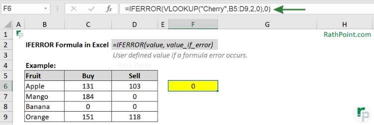
In the IFERROR formula, if you ignore the specified value and just add comma (,) then you will get zero (0) in case of error.
=IFERROR(VLOOKUP(“Cherry”,B5:D9,2,0),)
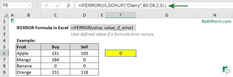
IFERROR formula Example (value)
Example 4 (nested IFERROR formula)
You can use the nested IFERROR formula in multiple formulas to meet the conditions. In the below example of IFERROR formula, if there is no error in first VLOOKUP formula then it will go to the next VLOOKUP formula and if still the error occurs then you will get the specified text as “Not Available”.
=IFERROR(VLOOKUP(“Cherry”,B5:D9,2,0), IFERROR(VLOOKUP(“Mango”,B5:D9,2,0),”Not Available”))
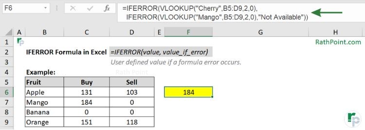
IFERROR formula Example (nested IFERROR formula)
Example 5 (empty)
In case you need the blank or empty cell as output then you need to keep the quotes without space as shown in the below Excel IFERROR example:
=IFERROR(VLOOKUP(“Cherry”,B5:D9,2,0),“”)

IFERROR formula Example (empty)
What are the Key Points for IFERROR Formula in Excel?
You must remeber the below key points while using the Excel IFERROR formula:
- The first step should be to check if any error in formula, before adding the IFERROR formula to it.
- If any of the argument is blank then the IFERROR formula considers it as empty string value and not an error, which is equal to double quote without space (“”) in formula and results as blank in cell.
- The Excel IFERROR formula can handle all errors due to formula such as #N/A, #VALUE!, #REF!, #DIV/0!, #NUM!, #NAME? and #NULL!.
- The IFERROR formula can replace errors with user defined text, number, another formula, or empty string.
- The IFERROR formula was introduced in Excel 2007, and it is available in all subsequent versions.
- To manage errors in Excel 2003 and old versions, you can use the ISERROR with IF formula.
- The alternative of IFERROR formula with limited error handing are:

How to use IFERROR Formula in Excel?
» Excel Home
» Excel Formulas
» Financial Formulas
» Logical Formulas
» Text Formulas
» Date & Time Formulas
» Lookup & Ref Formulas
» Math & Trig Formulas
» Statistical Formulas
» Engineering Formulas
» Cube Formulas
» Information Formulas
» Compatibility Formulas
» Web Formulas
